Applying the box-score paradigms from the NBA analytics community to the world of esports. A small adventure into using regularized adjusted ratings to get a gold standard and using statistical tools to approximate the resulting ratings. The canvas is the team modes in a competitive first person shooter called QuakeLive.

The basic approach will be to follow the steps at the backbone of most NBA analytics

1. Get a large dataset of players and matches. For this, a huge thanks to Eugene Molotov for QLLR. Additionally, database backups of the Russian QuakeLive community pickups are available with about 10,000 matches of TDM and CTF. derzkaya/KISA, upon request, provided me with the QLLR database from House of Quake with 32,000 matches of data from the recent EU pickup community.
2. Obtain estimates of player impact. The typical NBA approach is a method that adjusts for teammate and opponent quality. This is done through Regularized Adjusted Plus Minus (RAPM), which I’ll describe in further detail below.
3. Develop statistical measures that correlate with that impact. While player impacts ratings are nice, we’d like to estimate such ratings without having years of data to analyze at once. So we’ll build predictors for impact using only easily available measurements from each game. In this case, I’ll stick to the class of simple linear models to keep things interpretable and rein in model complexity.

Per usual, the code to do all the stats and make the graphs for this post is on GitHub.

For those of you unfamiliar to QuakeLive, welcome. It’s a PC first person shooter, a modest update to the 20+ year old Quake III. Players start with minimal equipment and collect various items that make their characters stronger; in the team mode TDM, players only survive an average of about 30 seconds. Core to the game is a mechanic called strafe-jumping (explained well in this video). If you’d like a feel for why fans of this genre stick with it, watch this highlight reel of gameplay.

Finding player impact

To rate all the players in the database we’re going to use Adjusted Plus Minus, whose classic article is Measuring How NBA Players Help Their Teams Win. Specifically we’ll add \(L_2 \) regularization and use cross-validation as in RAPM. In the NBA, most metrics target the 14y RAPM dataset from Jeremias Engelmann. If you’re an NBA fan and want modern RAPM numbers, I’d recommend NBAShotCharts from Ryan Davis. The best in-depth technical exploration is from Justin Jacobs, but I’ll give my own summary here.

In RAPM we make three key assumptions. One, we assume that a player’s impact is constant throughout the dataset; they don’t get better or worse. Two, we assume the impact of a player is linear. Three, players with little data should be regressed towards the mean. With these assumptions, finding player impact becomes solving a standard linear least-squares problem. For each game, we’ll create an equation of the form \[ \sum_{i \in T_1} x_i - \sum_{j \in T_2} x_j = S_1 - S_2 \] where \(T_1\) and \(T_2\) are the teams and \(S_1\) and \(S_2\) are the team’s scores. The \(x\) terms are the ratings for each player, which what we want to solve for. For a concrete example, for this game, we would have the equation \[x_{421} + x_{\text{pavel}} - x_{\text{proZaC}} - x_{\text{luminus}} = 97-91 = 6\] For each of the thousands of games in the dataset, we’ll have a equation like this. Compared to NBA analytics, where these equations are generated per possession, lineups in QuakeLive are constant throughout the game, so we only need one equation per match. Additionally, NBA analytics has a huge collinearity challenge as players have the same teammates for years. In the wonderful world of pickup games, teams are often random and we get much better coverage to isolate individual players’ impacts.

Now onto the small technical details. First, I’ll apply this to 4v4 Team Deathmatch (TDM) and 5v5 Capture the Flag (CTF) separately. I’ll filter out games which ended too quickly or got abandoned. In TDM this gives me about 13,000 games and 860 players. In CTF it’s about 7,000 games and 500 players. Using only the last year of data, I get about 5,000 games for each mode. Second, we will apply regularization, which encourages players with less data to be rated as average. The amount of regularization will be chosen with cross-validation, but I’ll often multiply it by a factor of 2 to 4 to keep the top10 from having players with only a handful of matches. Lastly, consider three choices of metric: score difference (\(S_1 - S2\)), score fractional difference (\( \frac{S_1 - S2}{S_1 + S_2}\)), and binary (\( 1[ S_1 > S_2 ] \)). For TDM, I’ll use fractional differences as total scores can vary wildly based on the map. For CTF, I’ll use binary loss as I’m less confident that score differences are meaningful. With binary loss, you can encode wins as +1 and -1, while retaining linear least squares. Or you can encode as 1 and 0, and switch to cross-entropy loss, giving you a version of logistic regression. I chose the latter, thereby giving you probabilities of victory via \( \sigma(X) = \frac{1}{1 + e^{-X} }\) where \( X \) is the difference of both teams’ summed player ratings.

Which players have the best impact?

The results of these regressions I’ll be calling adjusted net (aNet) in the case of TDM and adjusted wins (aWin) in the case of CTF. Adjusted net is your expected margin of victory if you had 3 average teammates and 4 average opponents. Adjusted wins, when passed through \( \sigma(x) \), gives you your chance of winning a game with average teammates and opponents; it is proportional (factor of ~1.8) to standard deviations in a logistic, so a score of 1.8 means you should win ~85% of the time.

For those who just want the results, there’s 4 versions here: total_cv, year_cv, total_4cv, year_4cv corresponding to using either the total dataset or roughly the last year (400 days). Likewise, I’ll post results with the regularization chosen cv and four times that. I’ll include standard errors, thereby giving you some understanding for how uncertain the ratings are; typically differences of 2 or 3 SE are considered significant.

TDM: year_cv, total_cv, year_4cv, total_4cv

CTF: year_cv, total_cv, year_4cv, total_4cv

One way to evaluate give confident ratings is to sort everyone by their lower end of their 95% confidence interval. Here’s that table for TDM over the total dataset.

alias	95% aNet
winz	29.03
abso	18.82
gogoplata	18.10
krysa	18.02
gainon	17.36
SPART1E	17.23
antonio_by	16.93
Cheddar Cheese Puffs	16.10
Xron	15.70

Compared to the currently HoQ Leaderboard, the 95% aNet from the past year matches the top 3 exactly and the top 10 are all in the top 15 in the leaderboards, so I’d claim this worked rather well. Similarly, the TrueSkill ratings on HoQ are pretty accurate!

alias	95% aWin
cockroach	1.57
MASTERMIND	1.56
ph0en|X	1.50
fo_tbh	1.35
jcb	1.25
Silencep	1.24
abso	1.16
Raist	1.08
MAKIE	1.06

For the CTF players the match against HoQ Leaders is pretty good again.

What do good TDM players do, on average?

While it’s great to have some robust ratings using years of data, that doesn’t give us much information about games themselves. So let’s follow the approach taken by many modern NBA statistics, such as Basketball Reference’s BPM, 538’s RAPTOR and Kev’s DRE. These are all in the class of Statistical Plus Minus (SPM): start with large-scale RAPM data and then build statistical models to estimate which box score numbers are predictive of good RAPM performance.

Starting with descriptive statistics, let’s go over the basic correlations. The x axis will be adjusted net (aNet) from total_4cv. We’ll have best-fit regression lines and Pearson’s R shown. For all of these statistics, they’re adjusted based on the total score of the game to handle map & time variation. Specifically, all statistics are scaled so the total score of both teams would be 313 points (which is the average total across the dataset). All of these graphs show results for players with at least 100 games played.

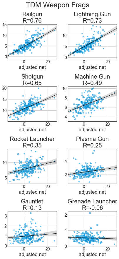
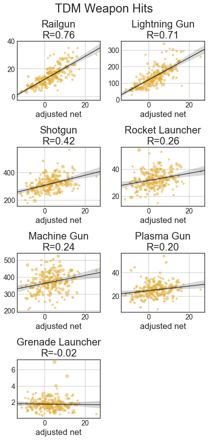
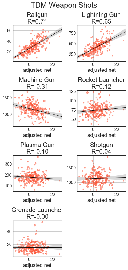
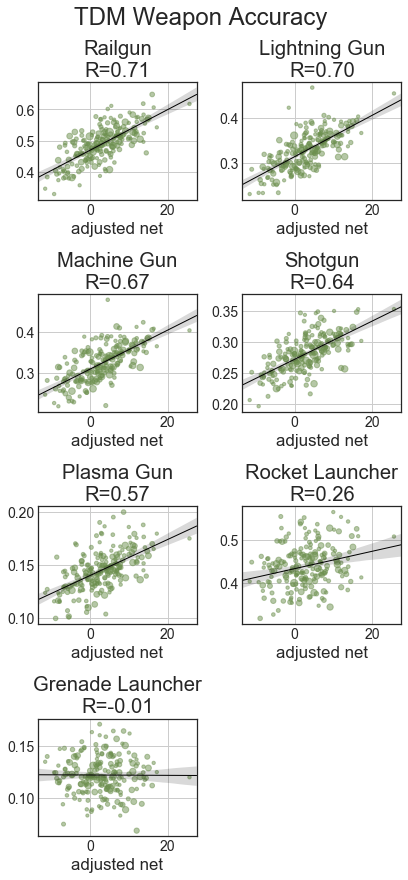
With the weapon statistics, we can see that across all categories, railgun and lightning gun statistics are strongly correlated with better players. With fragging, good players get a lot with RG, LG, SG, and MG, while RL and PG have weaker relationships and Gauntlet and GL kills are largely uncorrelated. Hits are like frags, just with weaker relationships, especially MG and SG. With usage, good players use a lot of LG and rail, while weaker players use a lot of MG and the other weapons are uncorrelated. Except for RL and GL, accuracies with weapons are well correlated with better players.

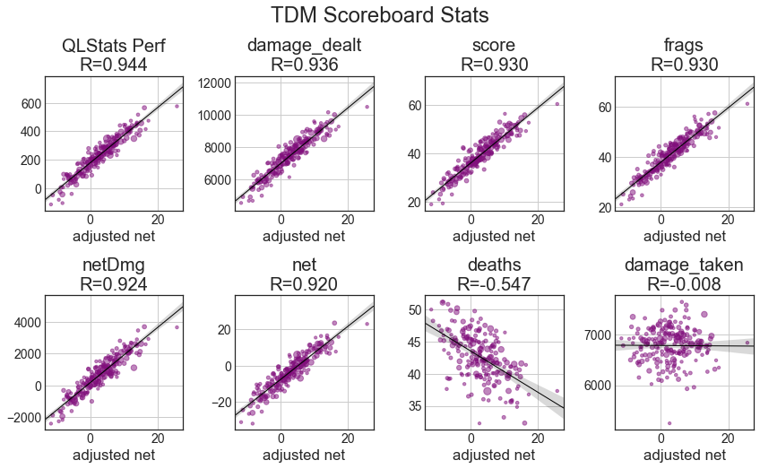
With the scoreboard stats, I’ve added QLStats’ TDM Perf rating, which is 5*net + 4*netDmg/100 + 3*dmgDone/100, which turns out to correlate really well on average. I suspect measurements like frags and damage_dealt are more predictive of good players than net and netDmg because they reward activity. That is, hiding in a corner and avoiding players may preserve your score, but it might tank your teams’ performance. Damage taken has no correlation, as more active players will pickup items.

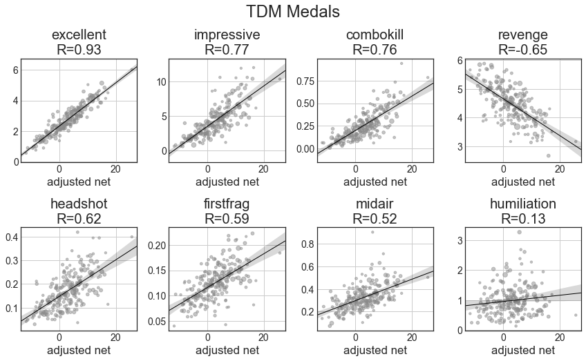
Amusingly, the medals have some of the highest correlation of player impact of any statistic. Excellent (2 frags in 2 seconds) is a wonderful predictor of performance. Likewise, revenge (frag someone who fragged you 3 times in a row) correlates with poor performance. Some of the others, such as midair and firstfrag may just be indicative of general combat ability and correlate reasonably well with impact.

So which features really matter? One way to measure feature importance is gain in decision forests, which tells us how much accuracy boost comes from using a specific variable to make decisions. More than 90% of the gain comes from splitting on score 0.34, damage_dealt 0.16, netDmg 0.14, frags 0.1 and net 0.1. Another way to to train a cross-validated linear predictor on normalized features and see where differences from average are most important. Here the results are excellent 1.33, score 1.03, net 1.02, netDmg 0.84, mg_frags 0.63, damage_dealt 0.53, impressive 0.41 and frags 0.37.

Ultimately, you can get a good predictor in lots of ways, as many feature are well correlated with performance. Using all the players, weighted by games played, instead of just those with > 100 games played, we can obtain a formula roughly like ( score / 3.3 ) + ( excellent * 3.0 ) + ( damage_dealt / 487.2 ) + ( mg_frags / 1.3 ) + ( deaths / -4.4 ) + ( lg_hits / 48.9 ) + ( rg_hits / 4.3 ) + ( revenge / -1.0 ) for Statistical Net (sNet) and this predicts aNet very well. Although, even QLStats Perf does a good job, I think you could improve the weights to score + ( damage_dealt / 181.2 ) + ( deaths / -3.5 ) + ( damage_taken / -275.1 ).

What do good TDM players do, in a particular game?

To me, the above analysis had a glaring flaw. While the impressive medal may have a 0.78 correlation with performance, medals in general have high variance. So while railgun hits has a slightly worse 0.76 correlation, it is likely a more reliable indicator from a given match. For example winz averages 6.0 ±3.1 excellent medals in 85% of games, but 61 ±10.4 frags. If they have roughly equal predictive power on average, you’d prefer the one that is lower variance.

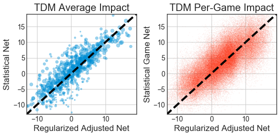
So instead we’ll build a different regression. Instead of using a player’s average statistics across all their games, we’ll try to predict their aNet from any particular game of theirs. There resulting statistic I’ll call sgNet for Statistical Game Net.

And here is where we all the statistical power gives us something that’s a little more reliable than existing metrics

	aNet R from per-game
excellent	0.405
net	0.533
netDmg	0.569
damage_dealt	0.638
QLStats	0.642
sNet	0.643
sgsNet	0.721
sgNet	0.741

The formula for sgNet is pretty complicated so instead I made a simpler version called sgsNet which is just (( frags / -3.75 ) + ( score / 3.9 ) + ( mg_hits / 55.34 ) + ( lg_hits / 160.48 ) + ( damage_dealt / 380.15 ) + ( mg_shots / -158.56 ) + ( deaths / -20.03 ))

Unfortunately I can’t really parse the huge formula for sgNet which is (( damage_dealt / 756.4 ) + ( damage_taken / 535.7 ) + ( frags / -6.2 ) + ( deaths / -22.9 ) + ( score / 5.0 ) + ( net / 8.9 ) + ( netDmg / 1731.3 ) + ( excellent / 10.9 ) + ( headshot / -7.5 ) + ( impressive / -122.2 ) + ( revenge / -50.1 ) + ( humiliation / -6.0 ) + ( midair / 2.9 ) + ( combokill / 8.5 ) + ( firstfrag / 24.0 ) + ( rampage / -1.0 ) + ( perforated / -1.1 ) + ( quadgod / -0.4 ) + ( gl_frags / -4.3 ) + ( gl_hits / -24.5 ) + ( gl_shots / 23.3 ) + ( gt_frags / 24.3 ) + ( lg_frags / -8.2 ) + ( lg_hits / 62.3 ) + ( lg_shots / -267.4 ) + ( mg_frags / -17.1 ) + ( mg_hits / 62.7 ) + ( mg_shots / -183.6 ) + ( pg_frags / -5.0 ) + ( pg_hits / 78.5 ) + ( pg_shots / -2521.2 ) + ( rg_frags / -3.7 ) + ( rg_hits / 13.6 ) + ( rg_shots / 38.3 ) + ( rl_frags / -4.6 ) + ( rl_hits / -48.3 ) + ( rl_shots / 42.9 ) + ( sg_frags / -8.2 ) + ( sg_hits / 272.6 ) + ( sg_shots / -663.1 ))

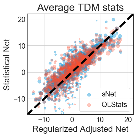
If you’d like to see these metrics (with sgsNet as the sgNet), you can find the table of results for the tdm_total dataset at this location. The graph at the top of this post is a visualization for those results.

Players with a low sgNet/sNet but a high aNet may be players with a lot of teamwork intangibles that don’t show up in the basic statistics. Players like abso and clawz clearly put up huge stats and their statistical indicators are as good as their aNet, while a players like krysa and pecka have lower statistical indicators but still help their teams win.

The CTF Section

We’ll mostly follow the methods & models used for TDM above. For details refer there.

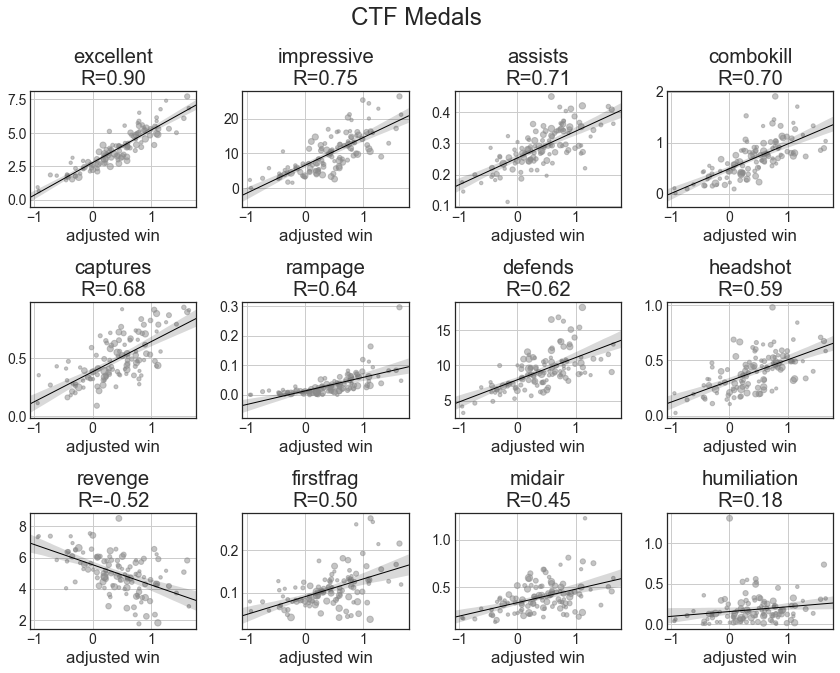
Once again, the combat medals of excellent and impressive dominant, more so than even captures

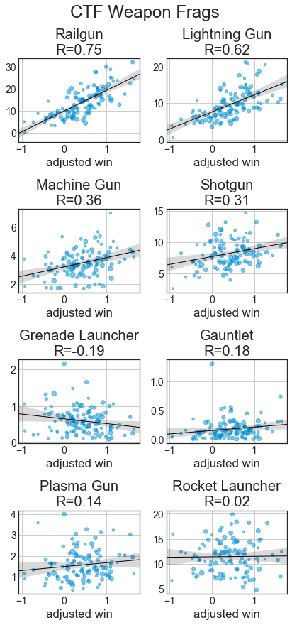
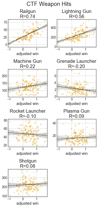
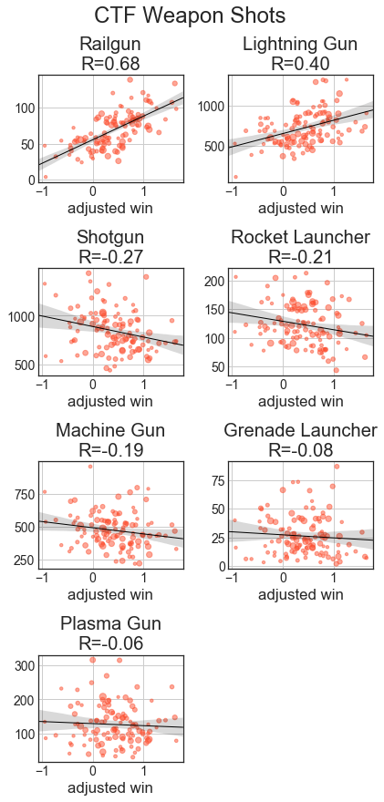
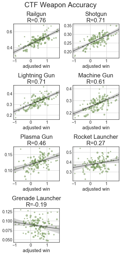
Once again, railgun and lightning gun dominate the charts. Rocket, Plasma and Grenades have nearly no correlation as they begin to be used for far more spam. Grenade launcher accuracy has a decent negative(!) correlation with impact, as top players spam it so much. Weapon availability isn’t a huge issue for defenders, so the Hits/Shots stats become much less predictive than they were in TDM.

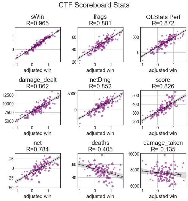
In the scoreboard stats, on average, the QL Stats Perf calculation of clip(damage_done/damage_taken,0.5,2) * (score + damage_done/20) works a little better than netDmg. Damage taken has nearly no correlation, and deaths have a weaker correlation in CTF than they did in TDM. net also has less value than most other stats.

The QLStats formula performs worse in CTF across the entire set of players (instead of only those with 100+ games as shown in the graphs), having a correlation of only 0.658 while sWin is at 0.667. The formula for sWin in this case is ( score / 32.62 ) + ( damage_dealt / 1387.75 ) + ( captures * 4.61 ) + ( excellent / 1.0 ) + ( mg_hits / 74.63)

Lastly come the per-game predictions, seen below.

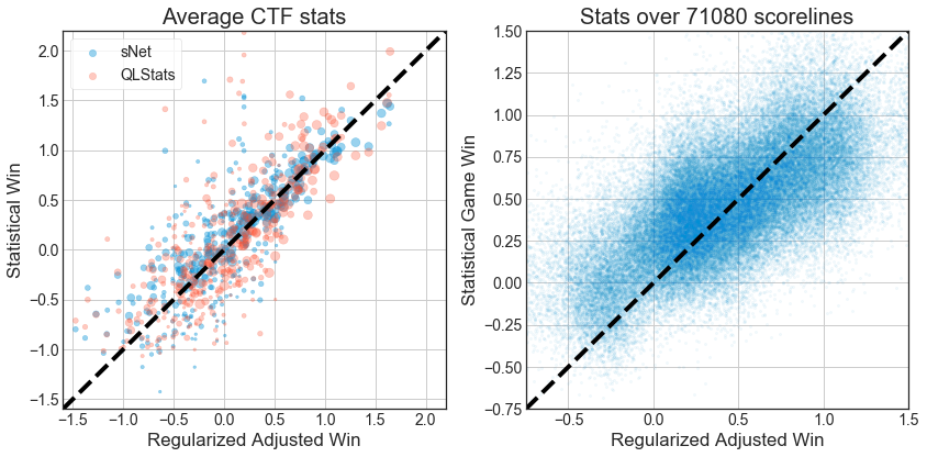
There is a notable improvement from building a per-game predictor (sgWin) instead of an average stats predictor . Even the simplified version (sgsWin) is pretty good and the formula is (( deaths / -1.0 ) + ( lg_shots / -37.08 ) + ( damage_dealt / 114.61 ) + ( sg_shots / -38.39 ) + ( lg_hits / 12.53 ) + ( sg_hits / 10.91 ) + ( damage_taken / 168.9 ) + ( mg_hits / 9.23 ) + ( mg_shots / -33.5 ) + ( score / 32.45 )). Interesting there seems to be a focus on combat skills.

	aWin R from per-game
net	0.459
damage_dealt	0.535
excellent	0.415
sWin	0.524
netDmg	0.560
QLStats	0.583
sgsWin	0.684
sgWin	0.702

Interestingly, sWin does worse than the QLStats Perf metric on individual games, even though it performed better in aggregated statistics. It does even worse than netDmg! The full sgWin formula is again an uninterpretable mess, not worth the space.

You can find the table of all these metric results for all players in the ctf_total dataset at this location.